Getting started
First of all, download the source code of the Matlab toolbox.
Source code is hosted at Github.
To have more details about the use of the toolbox, please have a look to :
README.txt
How to use the GUI for “pop-in” analysis from indentation tests ?
First of all a GUI is a Graphical User Interface.
- Run the following Matlab script :
demo.m
- Answer ‘y’ or ‘yes’ (or press ‘Enter’) to add path to the Matlab search paths, using this script:
path_management.m
- The following window opens:
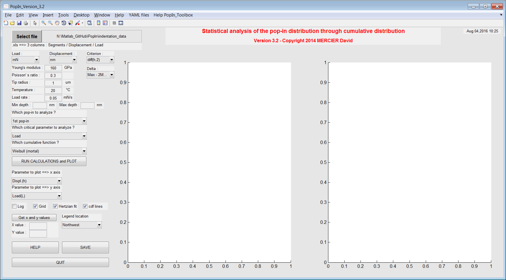
Figure 2 Screenshot of the main window of the PopIn toolbox.
- Import your (nano)indentation results (.xls file obtained from MTS software with at least more than 20 indentation tests for statistics), by pressing the button ‘Select file’.
- Select the end segment (if segments exist), in order to set the maximum indentation depth.
- Set units and criterion to detect pop-in.
- Once the dataset is loaded and parameters set, run calculations by pressing the green button ‘RUN CALCULATIONS and PLOT’.
- Load-displacement curves and selected cumulative distribution function (cdf) are plotted respectively on the left graphic and the right graphic.
- A picture of the main window as .png file is created and cdf fit results are stored in a .txt file when you press the button ‘SAVE’.
- Results are accessible by typing in the Matlab command window (here for 50 indentation tests) :
gui = guidata(gcf)

gui =
     config: [1x1 struct]                % config. of the GUI
     data_xls: [1x1 struct]              % details about .xls file
     handles: [1x1 struct]               % handles of the GUI = buttons, boxes...
     settings: [1x1 struct]              % settings of the GUI
     flag: [1x1 struct]                  % flags for errors, calculations
     data: [1x50 struct]                 % data cropped
     results: [50x1 struct]              % results obtained after calculations
     Hertz: [1x1 struct]                 % details about hertzian fit
     cumulativeFunction: [1x1 struct]    % cdf fit results
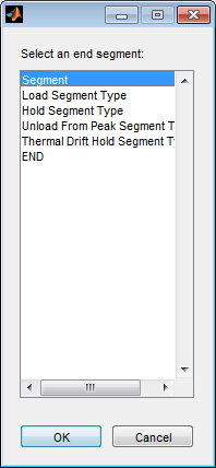
Figure 3 File selector.
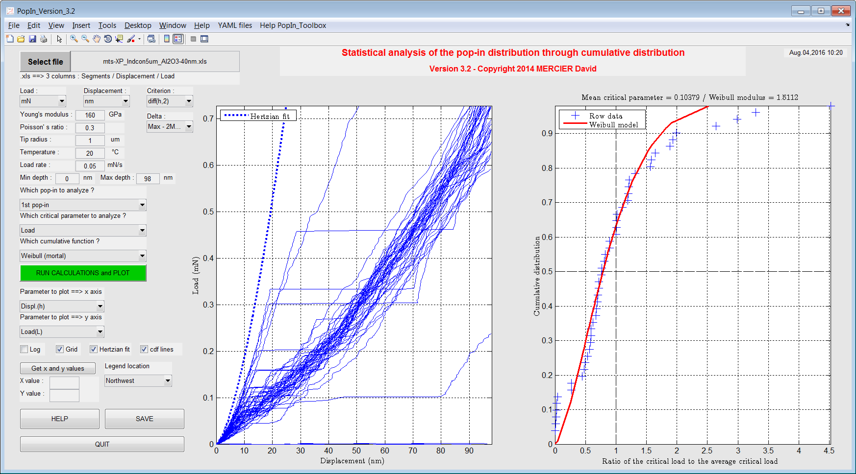
Figure 4 Plot of the load-displacement curves and the mortal Weibull cdf after loading of data.
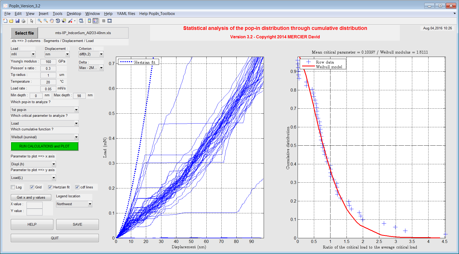
Figure 5 Plot of the load-displacement curves and the survival Weibull cdf.

Figure 6 Plot of the load-displacement curves and the mortal modified Weibull cdf (Chechenin’s model).
The YAML configuration files
Default YAML configuration files, stored in the folder yaml_config_files, are loaded automatically to set the GUI:
You have to update these YAML config. files, if you want to change indenter properties, constant parameters of models and constant parameters of the least-square method used to solve nonlinear curve-fitting and the path to your datasets.